Multi-species Dose, Varying Emissions
|
||||
 Previous |
|
|
 Next |
|


In a previous example, a time-invariant unit source calculation was used to demonstrate the dose calculation using CON2REM. In this case, following a similar procedure used previously to generate one model simulation for each emission period, we use CONDECAY with multiple species defined on the command line to create concentration files with multiple species for each emission time period from one computational species. CON2REM is then applied to convert the contents of each file to dose.
- The files required for the simulation (download to your work directory) are the same as the previous example but with two new additions:
wrf11031400.bin WRF meteorological data activity_unit.txt unit emissions and dose conversion factors for 10 radionuclides cfactors_all.txt time varying emissions for 10 radionucides dose_temit.sh Script for UNIX/Mac or ... dose_temit.bat Script MS-Windows
- Although more can be defined, a minimum of two pollutants are required to run this simulation. The simplest approach is to put both on the same computational particle. Add the additional variable line to the standard SETUP.CFG namelist file:
maxdim = 2, define two species on each computational particle - The simulations are scripted to be run sequentially for each release time. For each increment of the release time, the run duration would decrease by the same amount. We initially define the RUN variable to be 72 hours. In this example, only three days are simulated:
- run=72
- Loop day: 14 15 16
- Loop hour: 00 03 06 09 12 15 18 21
- ... section to create the CONTROL file
- ... execute HYSPLIT
- ... decrement run by 3 hours
- The CONTROL file is dynamically created within the body of the script, setting the start time, run duration, and concentration output file name. The name of the concentration output file should reflect the release time TG_{MMDDHH}:
11 03 $DD $HH release start time 2 number of start locations 37.4206 141.0329 1.0 bottom of release layer 37.4206 141.0329 100.0 top of release layer $run run duration in hours ... additional CONTROL file lines TG_03$DD$HH output file name by release time - Ensure that the emission section of the CONTROL file is set to a unit hourly rate. Two entry sections are required, one for each computational species:
2 two pollutant definitions follow RNUC generic particulate radionuclide 1.0 emission rate units per hour 3.0 emission duration in hours 0 0 0 0 0 emission start time (0 defaults to run start) NGAS generic noble gas 1.0 emission rate units per hour 3.0 emission duration in hours 0 0 0 0 0 emission start time (0 defaults to run start) - The deposition section of the CONTROL file should be configured to correspond to the general characteristics of the particle radionuclide RNUC and noble gas NGAS pollutants:
2 two pollutant definitions follow 1.0 1.0 1.0 defined as a particle 0.001 0.0 0.0 0.0 0.0 forced dry deposition 0.1 cm/s 0.0 8.0E-05 8.0E-05 below and within cloud wet removal 0.0 no radioactive decay 0.0 no resuspension 0.0 0.0 0.0 defined as a gas 0.0 0.0 0.0 0.0 0.0 no dry deposition 0.0 0.0 0.0 no wet removal 0.0 no radioactive decay 0.0 no resuspension - Once the HYSPLIT unit source calculations have been completed, five steps are required to convert from unit source air concentrations and deposition to a top-ten radionuclide dose calculation.
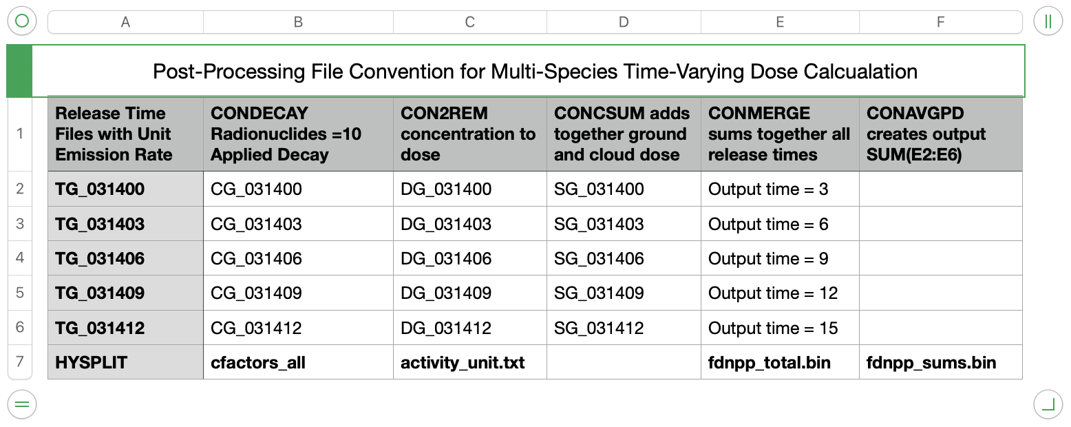
- The multi-file TCM structure uses the program CONDECAY to apply a time-varying release rate as defined in the cfactors_all.txt file to the twenty four TG_03{DDHH} processed files. The program reads these files and associates the column number in the emissions file with the species index number in the HYSPLIT file and applies radioactive decay from the decay start time according to the half-life specified. In this application CONDECAY has 10 radionuclide species defined on the command line; which means that each TG dispersion coefficient can generate 10 species in the output file using the emission rates defined in cfactors_all.txt. In this example, the emission rates are the ones used by UNSCEAR for their assessment of the Fukushima accident. Note that the activity.txt used in the previous section shows the maximum emission rate value for each species as tabulated in the cfactors_all.txt file.
condecay apply emission rates to multiple files -1:1:11025.8:C137 column 1 = species 1 = 11025.8 da = Cs-137 -3:1:8.02330:I131 column 3 = species 1 = 8 da = I-131 -4:1:754.020:C134 column 4 = species 1 = 754 da = Cs-134 -5:1:0.86958:I133 column 5 = species 1 = 1 da = I-133 -6:1:1.10167:B140 column 6 = species 1 = 1 da = Ba-140 -7:1:1.44980:L140 column 7 = species 1 = 1 da = La-140 -8:1:3.23000:T132 column 8 = species 1 = 3 da = Te-132 -9:1:2.18000:A110 column 9 = species 1 = 2 da = Ag-110m -10:1:3.0200:NB95 column 10= species 1 = 3 da = Nb-95 -14:2:5.2474:X133 column 14= species 2 = 5 da = Xe-133 +t031106 decay start time (when fission stopped) +ecfactors_all time varying emission rate file +iTG_ input file prefix (wild card processing) +oCG_ output file prefix (for each input file) - The next step involves processing each CG concentration file and matching it to the same radionuclide ID (-s1 option in con2rem) in the dose conversion factor file and then compute the dose. A customized dose conversion factor file was created called activity_unit.txt which contains a row for each of the 10 radionuclides in the emissions file using the same 4-character label and where all the emission rates have been set to a unit value. The actual emission rates and decay is not applied in this step (option -t0) because they were applied in the previous step.
con2rem convert concentration to dose -iCG_03{DDHH} HYSPLIT binary output file -oDG_03{DDHH} binary output dose file -aactivity_unit.txt unit emission rates and dose factors -s1 match species in activity.txt with the input file -t0 do not apply decay -d1 compute dose over averaging period - After each conversion to dose, the ground-shine and cloud-shine dose values are added together each time period into a combined total dose output.
concsum add ground- and cloud-shine -iDG_03{DDHH} input binary dose file -oSG_03{DDHH} output binary total dose file -l combine ground- and cloud-shine -pDOSE species output label - The next step is to merge the individual release dose files into a single file representing the dose from all releases using the program CONMERGE. The final result is a single file fdnpp.bin that contains all releases and sampling periods using the defined emission profile.
- dir /b SG_??????.bin >merg_list.txt
- conmerge -imerg_list.txt -ofdnpp_total.bin
- In the last post-processing step, the 3-hourly dose values are summed together to obtain a total dose over the specified averaging time period:
conavgpd average or sum over time -ifdnpp_total.bin input file of 3-h dose values -ofdnpp_sums.bin binary output file of summed doses -a11031400 YYMMDDHH of summation start -b11031700 YYMMDDHH of summation end -r1 r=1 to sum or r=0 to average - For the first graphics, we produce a time series of the sum of the ground- and cloud-shine dose one would receive at Tokai-mura, about 100 km south of the Fukushima plant. The numbers shown represent the dose each 3-h period and must be accumulated for the total dose:
echo Tokai 36.4356 140.6025 >latlon.txt location to file con2stn extract time series at a location -ifdnpp_total.bin binary dose output file -oTokai.txt text output file at location -slatlon.txt latitude & longitude for each location timeplot time series plot -iTokai.txt input file with data to plot -p2 plot points and connecting lines -y log axis scaling 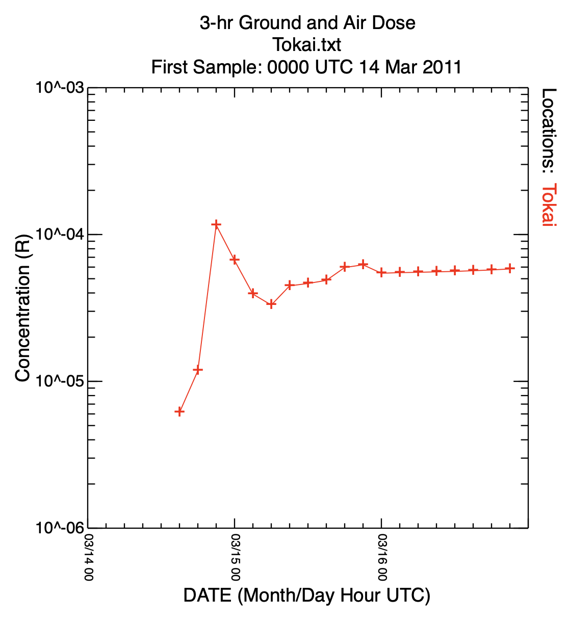
- In the last graphic, we plot the accumulated dose, computed previously, over the entire model simulation period:
concplot concentration plotting program -ifdnpp_sums.bin binary input of dose summation -odose_plot Postscript output file -c4 force contour levels -v1.0+0.3+0.1+0.03+0.01+0.003+0.001 set forced contours 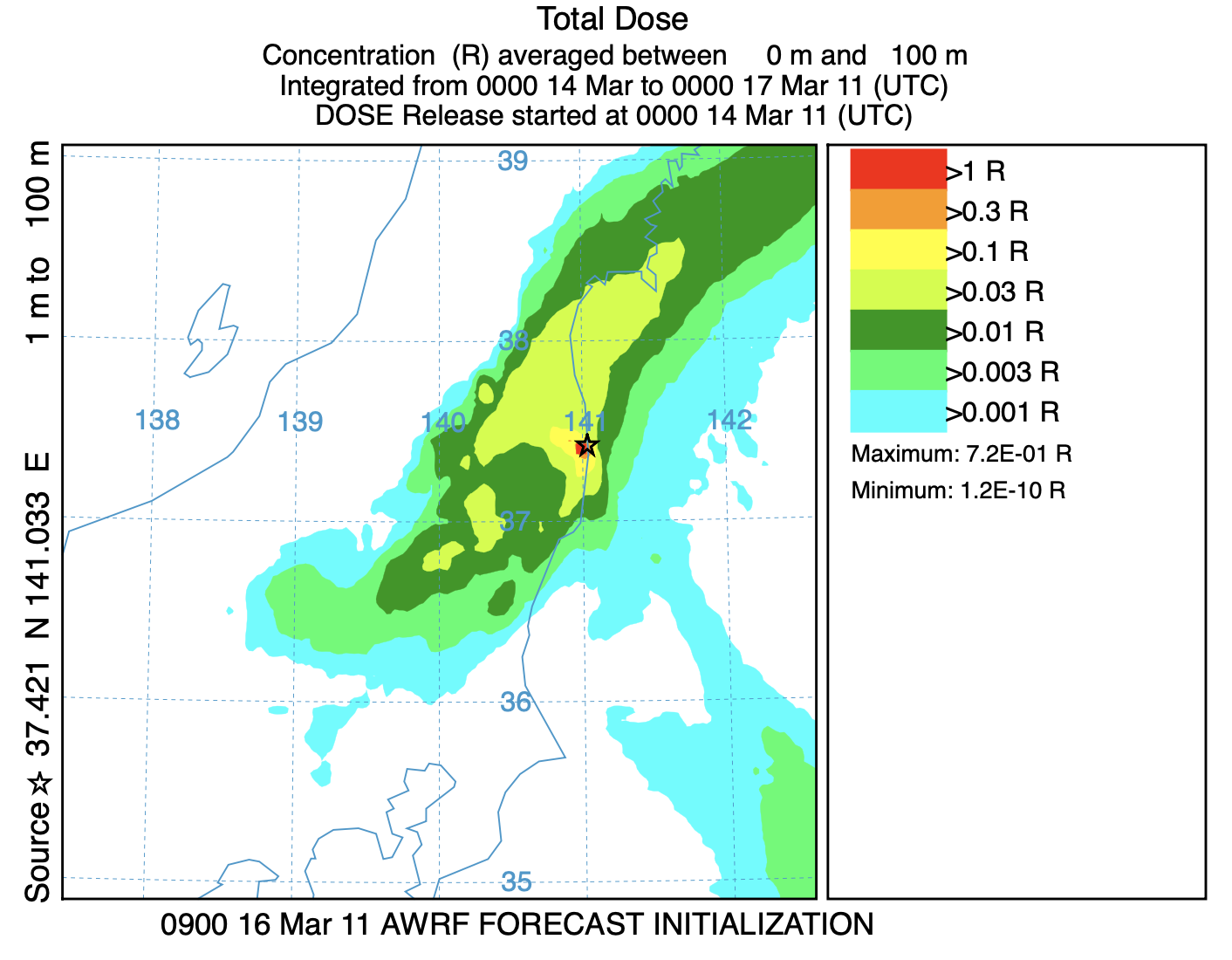
In this HYSPLIT radiological configuration, a unit source dispersion-deposition calculation with two computational species, one representing a small particle and other a noble gas, were run for each emission period over the duration of the period of interest. Post-processing programs were used to assign each computational species to multiple radionuclides, each with its own emission rate, decay, and dose factors, to compute dose. The resulting doses using realistic time-varying emissions were much smaller than the calculation using a constant maximum emission rate.