Multi-file Transfer Coefficient Matrix
|
||||
 Previous |
|
|
 Next |
|


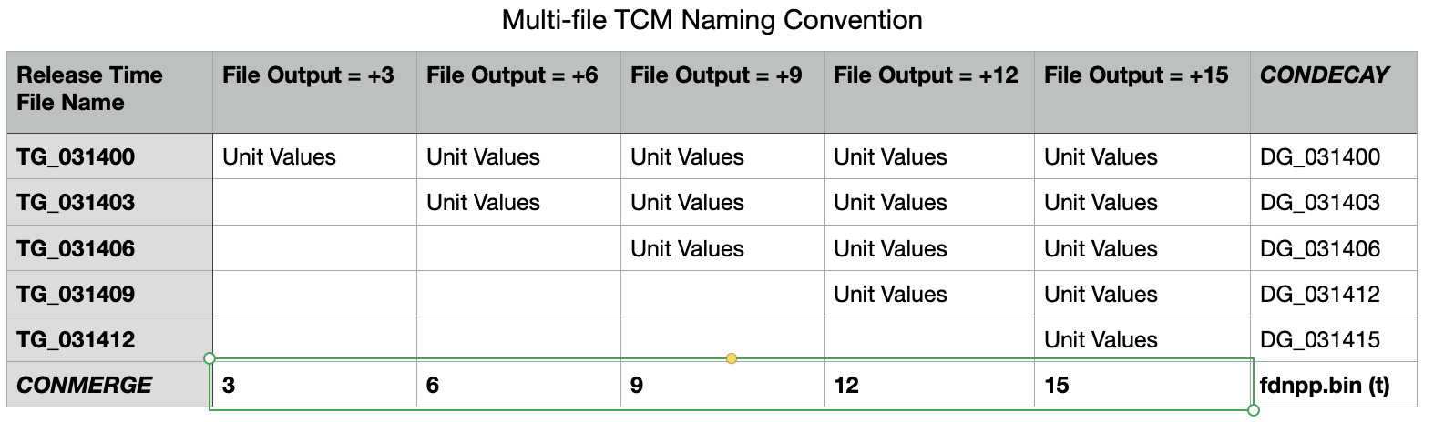
When each emission period is its own independent calculation, the results can be organized in matrix form such that we can represent each emission time as a row and the concentration grid as a column. Then the column sum over all rows represents the total calculated concentration for all emissions while the row sum represents the contribution of that emission period to each output time. The transfer coefficient matrix represents the fractional contribution of each emission time to each output time period. We can multiply the coefficient values for each row by its source term to obtain the calculated air concentration and deposition values. Multiple source term scenarios can be investigated without rerunning the dispersion model.
- The files required for the simulation (download to your work directory) are the same as the previous example:
wrf11031400.bin WRF meteorological data JAEA_C137.txt Cs-137 measurements at Tokai-mura cfactors.txt hourly radionuclide emissions (replaces EMITIMES) tcm_file.sh Script for UNIX/Mac or ... tcm_file.bat Script MS-Windows
-
There are several approaches to computing the TCM. An automated method was demonstrated previously where multiple emission periods were configured in one simulation, but with a one species limitation. To overcome this restriction, a multi-file approach is required. In this case, the model is run with a three hour emission period and subsequent simulation starts three hours later and has a simulation duration of three hours less than the previous one. All simulations have a unique output file where the name indicates the start time of the emission (TG_{MMDDHH}).
- Because each 3-h release period is represented by one simulation, if only 2500 particles per hour are released, the maximum number of particles followed in any one simulation would be 7500. The SETUP.CFG namelist file should contain:
numpar = -2500, particle release rate per hour (negative) maxpar = 10000, maximum particle number per simulation - The simulations are scripted to be run sequentially for each release time. For each increment of the release time, the run duration would decrease by the same amount. We initially define the RUN variable to start at 72 hours and reduce the run time by 3 hours for each new simulation that starts 3 hours later.
- run=72
- Loop day: 14 15 16
- Loop hour: 00 03 06 09 12 15 18 21
- ... section to create the CONTROL file
- ... execute HYSPLIT
- ... decrement run by 3 hours
- The CONTROL file is dynamically created within the script, setting the start time, run duration, and concentration output file name. The name of the concentration output file should reflect the release time TG_{MMDDHH}:
11 03 $DD $HH release start time 2 number of start locations 37.4206 141.0329 1.0 bottom of release layer 37.4206 141.0329 100.0 top of release layer $run run duration in hours ... additional CONTROL file lines 1 one pollutant CPAR defined as a Cesium Particle 1.0 emission rate of one units per hour 3.0 emission duration 3 hours each cycle ... additional CONTROL file lines TG_03$DD$HH output file name by release time - The multi-file TCM structure uses the program CONDECAY to apply a time-varying release rate to the twenty four TG_03{DDHH} processed files. The program reads these files and associates the column number in the emissions file with the species index number in the HYSPLIT file and applies radioactive decay from the decay start time according to the half-life specified. Using this approach, multiple species can be processed. In addition, for a single species within the HYSPLIT input file, multiple species can be written to the output file, one output species for each group (- prefix) defined on the command line. Other arguments use the + prefix. Output file names default to DG_03{DDHH}. In this particular case, we use column #1 of the cfactors.txt emission file:
condecay apply emission rates to multiple files -1:1:11025.8:C137 emission column 1 = species 1 = 11025.8 days = Cs-137 +t031106 decay start time (when fission stopped) +ecfactors emission rate file (.txt implied) +iTG_ input file prefix +oDG_ output file prefix - The final step is to merge the individual release files into a single file using the program CONMERGE. The procedure is similar to the CONAPPEND application. The final result is a single file fdnpp.bin that contains all releases and sampling periods using the defined emission profile.
- dir /b DG_?????? >merg_list.txt
- conmerge -imerg_list.txt -ofdnpp.bin
- In the first post-processing step, the model predicted concentration time series at Tokai-mura, about 100 km south of the FDNPP, is compared with the measurements:
c2datem convert model output to DATEM format -ifdnpp.bin HYSPLIT binary output file -oTokai.txt HYSPLIT DATEM output at Tokai -mJAEA_C137.txt measured data file in DATEM format -c1000.0 conversion from Bq to mBq -z2 select level #2 from input file 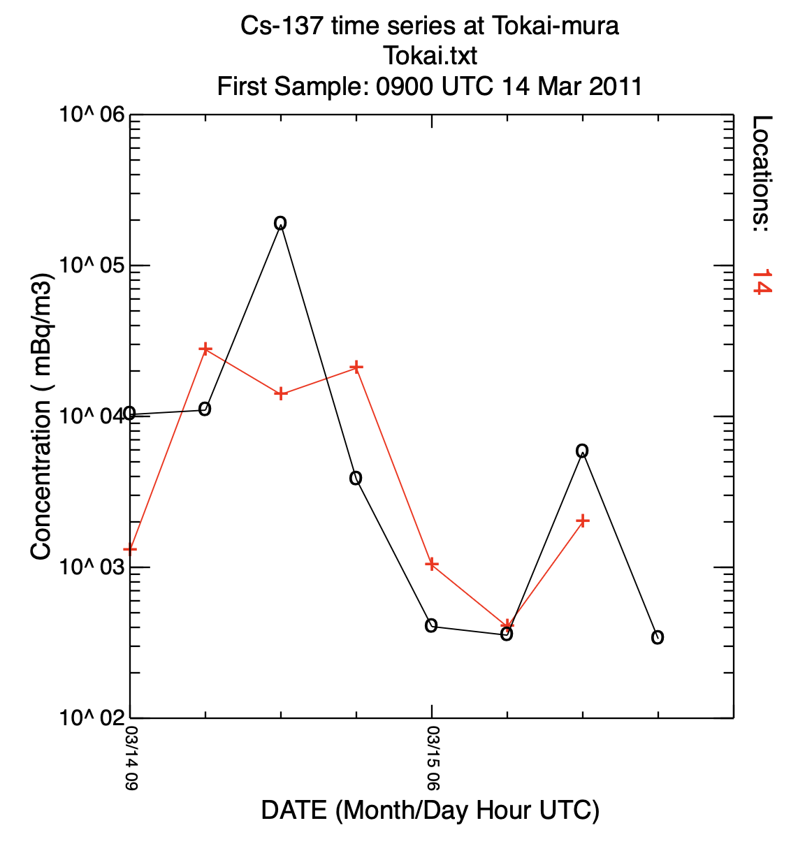
- In the second post-processing step, we create a plot of the total deposition:
concplot concentration plotting program -ifdnpp.bin HYSPLIT binary output file -oplot_dept Postscript output file -h37.0:140.0 location of map center -g0:100 radius of the map -y0.001 convert Bq to kBq -ukBq set units label on map -b0 -t0 process input data from bottom and top level 0 -k2 do not draw contour lines between colors -c4 force contour levels -v1000+500+200+100+50+20+10 set forced contours -r3 plot only the total accumulated deposition 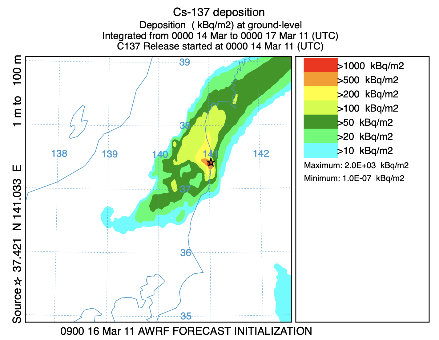
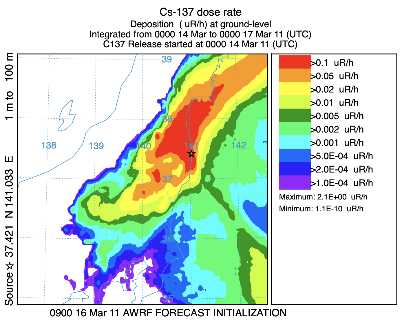
- In the last post-processing step we convert the air concentrations and accumulated deposition at each 3 hour output period to dose using the concentration plotting program. For this conversion we assume that the conversion factors are 3.3x10⁻¹¹ and 1.1E-12 (rem/h per Bq/m3 or per Bq/m2). Only the last time period is shown below:
concplot concentration plotting program -ifdnpp.bin HYSPLIT binary output file -oplot_dose Postscript output file -h37.0:140.0 location of map center -g0:100 radius of the map -x3.340E-05 convert air concentration to µrem/h -y1.08E-06 convert deposition to µrem/h -k2 do not draw contour lines between colors -c4 force contour levels -v0.1+0.05+0.02+0.01+0.005+0.002+ 0.001+0.0005+0.0002+0.0001 set forced contours -r2 sum dose (rate) each time period 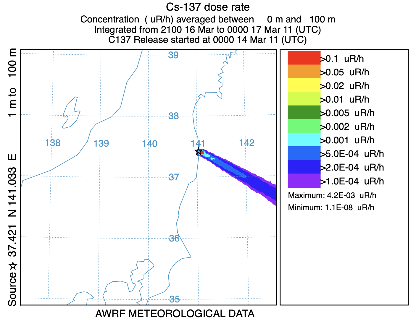
In the approach shown here, the TCM is constructed in such a way that there is one output file for each simulation and each simulation represents one release time. In contrast to the single file method, where one output file contains all release times, in the multi-file approach we can define multiple species in the same simulation, for instance a non-depositing gas, a depositing gas, and perhaps a small particle. Each species having its own deposition characteristics. These computational species could be associated with different radionuclides in the post-processing step.