A Single Transfer Coefficient Matrix
|
||||
 Previous |
|
|
 Next |
|


In a previous example we used the time-varying emission file EMITIMES to create realistic air concentration and deposition output. However, in some cases the emissions may be unknown and therefore it is necessary to run HYSPLIT in a way that the time-varying emissions can be applied as a post-processing step. In this way multiple emission scenarios can be tested and compared to measurements to find the best fit to the data without rerunning the dispersion calculation. In this simulation we will automatically divide the simulation into three hour emission periods, but the particles released during each emission period will be automatically tagged with a unique number (the pollutant index in the concentration array). Therefore, each release time will have its own element within the concentration array and within the same output file.
- Except for one new file to use instead of EMITIMES, the files required for the simulation (download to your work directory) are the same as the previous example:
wrf11031400.bin WRF meteorological data JAEA_C137.txt Cs-137 measurements at Tokai-mura cfactors.txt hourly radionuclide emissions (replaces EMITIMES) tcm_auto.sh Script for UNIX/Mac or ... tcm_auto.bat Script MS-Windows
- To run this calculation only a minor modification to the CONTROL and SETUP.CFG files is required. When emission cycling is defined then the emission index tag will be incremented every 3 hours when ICHEM is set to 10. This also forces the code to assign the particle's emission time tag to the pollutant index of the concentration array, thereby permitting the output to be separated by emission time. Customize the namelist file with the additional variables shown below:
qcycle = 3 , a new emission cycle starts every 3 hours ichem = 10, concentration array layer defined each cycle 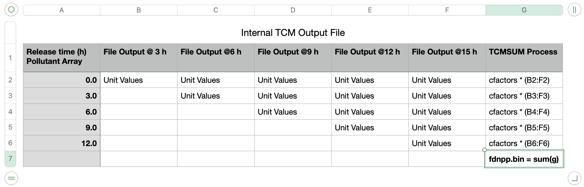
- The CONTROL file is almost identical to a standard simulation except that a unit emission (one per hour) for a duration of three hours should be specified:
1 one pollutant CPAR defined as a Cesium Particle 1.0 emission rate of one units per hour 3.0 emission duration 3 hours each cycle tcm.bin unique name for TCM output file - Run HYSPLIT:
${MDL}/exec/hycs_std single processor version - The program TCMSUM is used to apply a time-varying release rate to the unit-source multi-release time HYSPLIT output file. The TCMSUM program reads the HYSPLIT output file and associates column #1 of the cfactors.txt emission file with the unit source dispersion calculations for the appropriate emission times. The .bin suffix is automatically added to the end of the output file name. The half-life, decay start time, and output pollutant ID are defined on the command line:
tcmsum apply emission rates to unit source calculation -itcm.bin input file: HYSPLIT binary output file -ofdnpp binary output file corrected for emissions -t031106 start time (MMDDHH) for radioactive decay -h11025.8 half life in days for Cs-137 λ = log(0.5) / half-life Decay = exp(λt) -c1 select column #1 from the emissions file -scfactors.txt select name of the emissions file -pC137 pollutant ID label (4 characters max) - In the first post-processing step, the model predicted concentration time series at Tokai-mura, about 100 km south of the FDNPP, is compared with the measurements:
c2datem convert model output to DATEM format -ifdnpp.bin HYSPLIT binary output file -oTokai.txt HYSPLIT DATEM output at Tokai -mJAEA_C137.txt measured data file in DATEM format -c1000.0 conversion from Bq to mBq -z2 select level #2 from input file 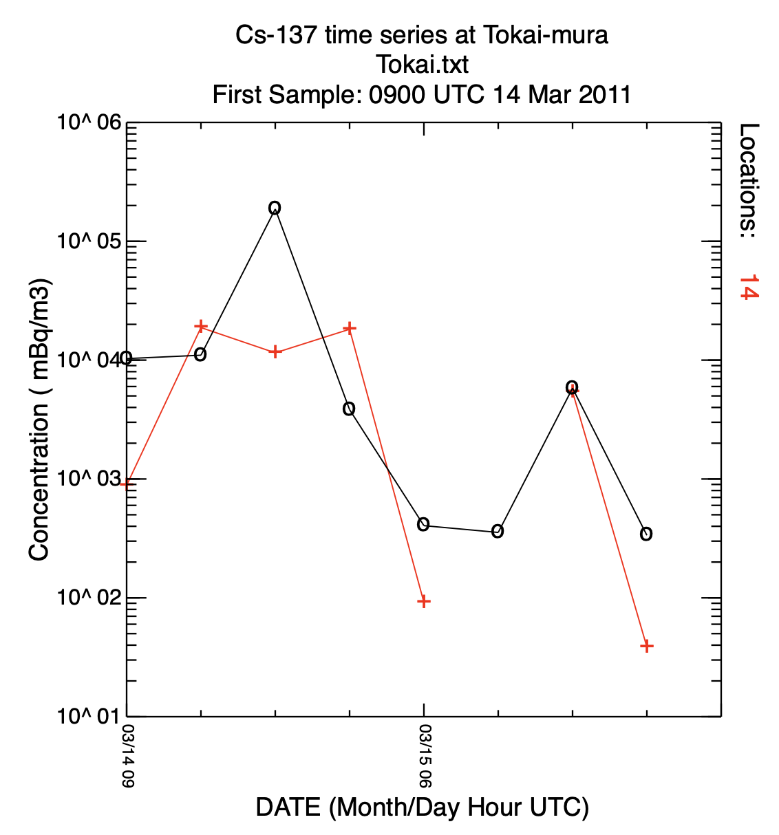
The result does have more variability than the previous simulation. In this situation, the release of more particles (10,000 p/h) provides a much more consistent time series, but at the cost of an increase in computational time. Clearly the greatest variability is in the prediction of the lowest concentrations. The mass per particle can have a substantial effect on the value of the calculated minimum concentrations. - In the second post-processing step, we create a plot of the total deposition:
concplot concentration plotting program -ifdnpp.bin HYSPLIT binary output file -oplot_dept base name of graphic output file +g1 output in SVG such that name={base}.html -h37.0:140.0 location of map center -g0:100 radius of the map -y0.001 convert Bq to kBq -ukBq set units label on map -b0 -t0 process input data from bottom and top level 0 -k2 do not draw contour lines between colors -c4 force contour levels -v1000+500+200+100+50+20+10 set forced contours -r3 plot only the total accumulated deposition 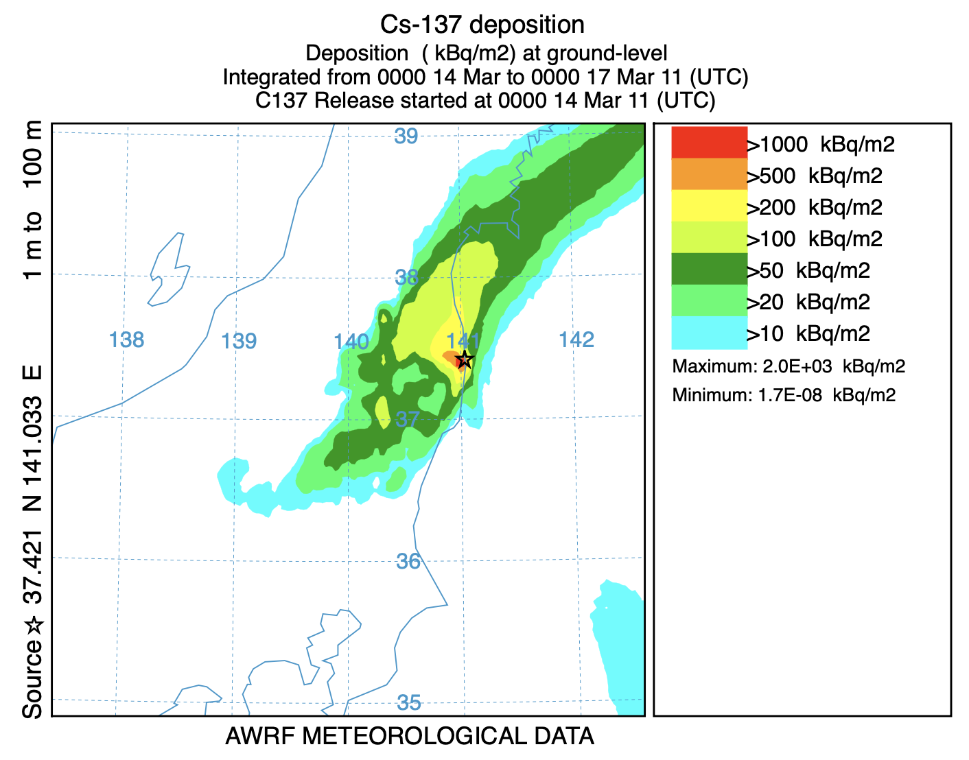
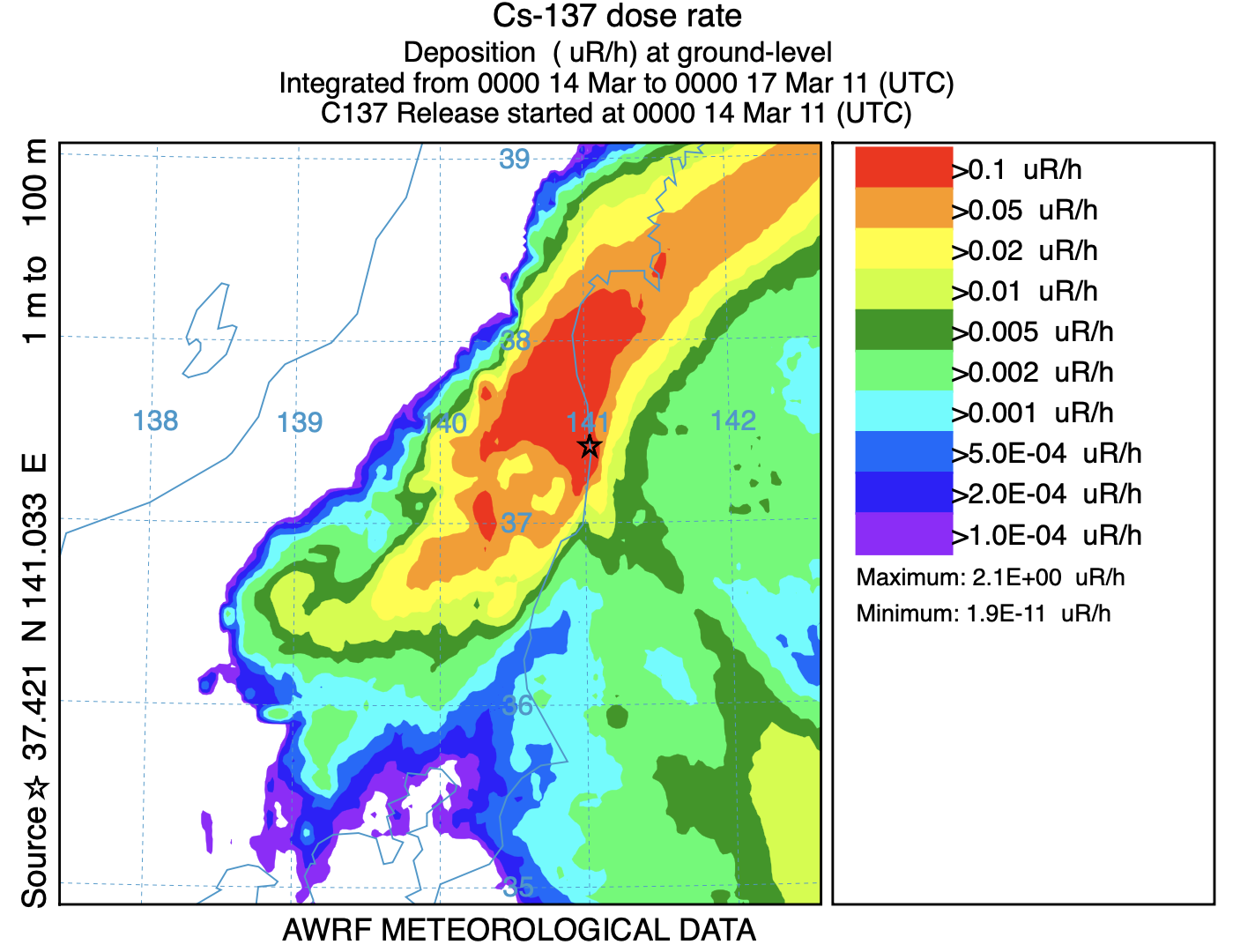
- In the last post-processing step we convert the air concentrations and accumulated deposition at each 3 hour output period to dose using the concentration plotting program. For this conversion we assume that the conversion factors are 3.3x10⁻¹¹ and 1.1E-12 (rem/h per Bq/m3 or per Bq/m2). Only the last time period is shown below:
concplot concentration plotting program -ifdnpp.bin HYSPLIT binary output file -oplot_dose base name of graphic output file +g1 output in SVG such that name={base}.html -h37.0:140.0 location of map center -g0:100 radius of the map -x3.340E-05 convert air concentration to µrem/h -y1.08E-06 convert deposition to µrem/h -k2 do not draw contour lines between colors -c4 force contour levels -v0.1+0.05+0.02+0.01+0.005+0.002+ 0.001+0.0005+0.0002+0.0001 set forced contours -r2 sum dose (rate) each time period 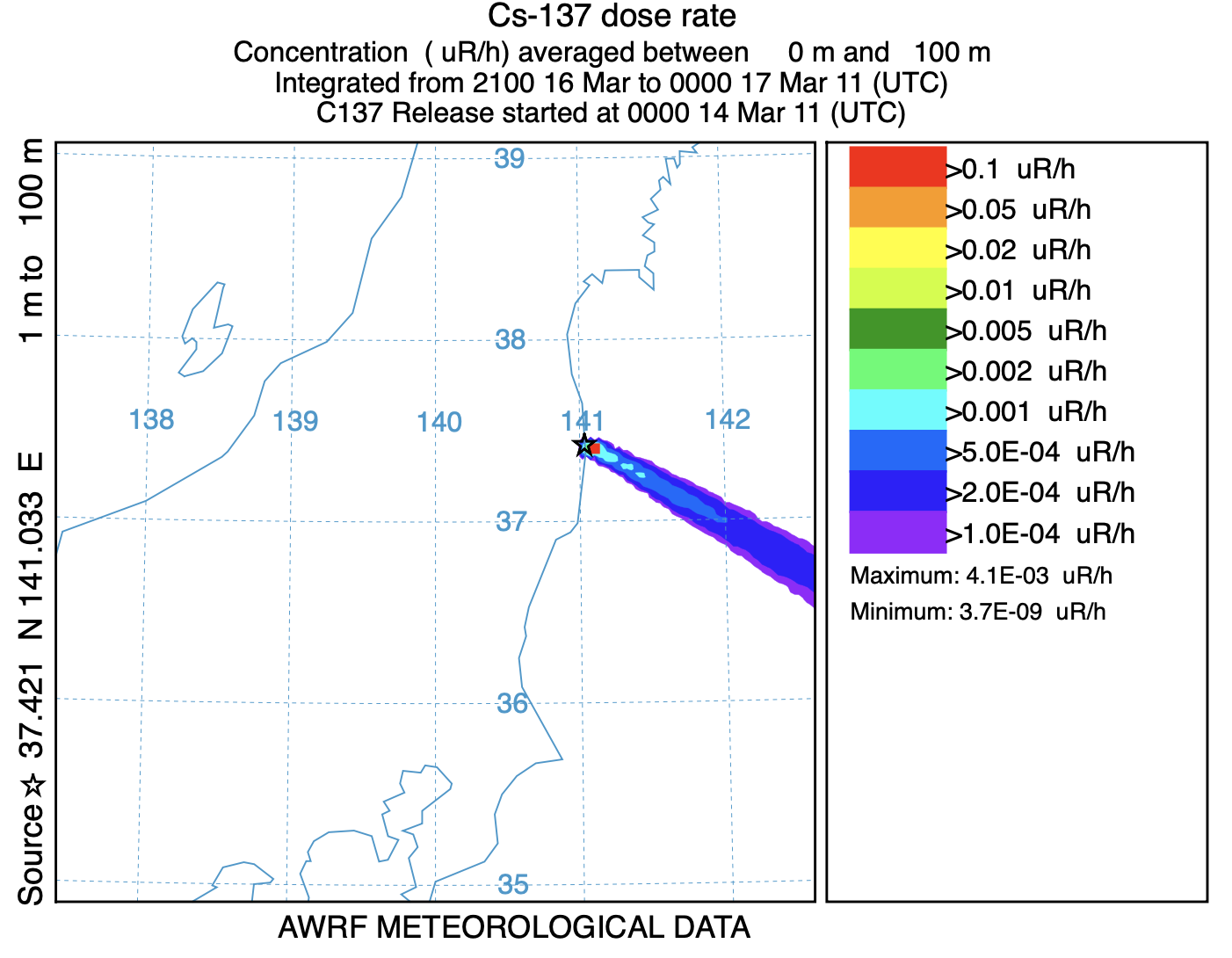
The approach outlined above is a quick and efficient method to create a transfer coefficient matrix (TCM) associated with different release times. A TCM is defined as the contribution of each source to each receptor location. Sources can vary in space, time, or both. The emission factors are applied after the simulation has completed. The limitation of this approach is that only one pollutant species is permitted during a simulation because the pollutant array index has been replaced by the emission time index. For more complex multi-species simulations, the multiple file approach is required.