Time Varying Emissions and Dose
|
||||
 Previous |
|
|
 Next |
|


In this example we define the time varying emission rate for Cs-137 during the most critical two-day period during the Fukushima accident to compute deposition and enter a simple conversion factor to estimate the dose for a single radionuclide. In the following sections below we review the key features of the script.
- Files required for the simulation (download to your work directory):
wrf11031400.bin WRF meteorological data JAEA_C137.txt Cs-137 measurements at Tokai-mura EMITIMES.txt hourly emissions of Cs-137 emit_time.sh Script for UNIX/Mac or ... emit_time.bat Script MS-Windows
You can edit the EMITIMES file if you have more recent emissions data. These emission data are based upon the UNSCEAR radionuclide inventory at the time fission stopped.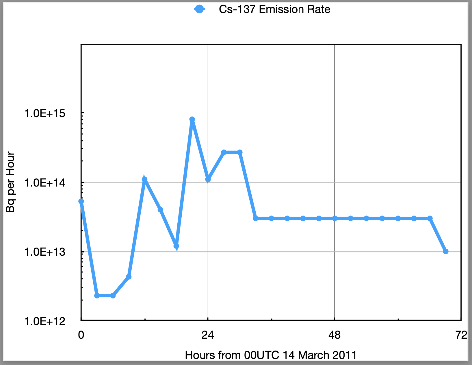
- Ensure that the emission section of the CONTROL file is set to zero to avoid using the wrong emission rate:
1 one pollutant CPAR defined as a Cesium Particle 0.0 emission rate units per hour 0.0 emission duration in hours - Configure the SETUP.CFG namelist file to optimize the calculation using WRF and to speed up the computation for quicker results by deleting particles that have moved off the domain of interest. The 2,500 p/h release rate was chosen as a compromise between obtaining faster results and still maintaining some fidelity to reality. Using finer resolution concentration grids in either space or time would require a larger particle release rate.
delt = 5.0, force time step khmax = 24, delete particles after 24h numpar = -2500, release 2500 per hour maxpar = 300000, maximum particle number efile = 'EMITIMES.txt', file with emission rates - Run HYSPLIT:
${MDL}/exec/hycs_std single processor version - In the first post-processing step, the model predicted concentration time series at JAEA site at Tokai-mura, about 100 km south of the FDNPP, is compared with the measurements:
c2datem convert model output to DATEM format -ifdnpp.bin HYSPLIT binary output file -oTokai.txt HYSPLIT DATEM output at Tokai -mJAEA_C137.txt measured data file in DATEM format -c1000.0 conversion from Bq to mBq -z2 select level #2 from input file timeplot plot a time series of values -iTokai.txt HYSPLIT output at Tokai in DATEM format -sJAEA_C137.txt supplemental DATEM file with measured data +g1 output in SVG to timeplot.html -p2 plot data points with connecting line -y log scaling of the y-axis 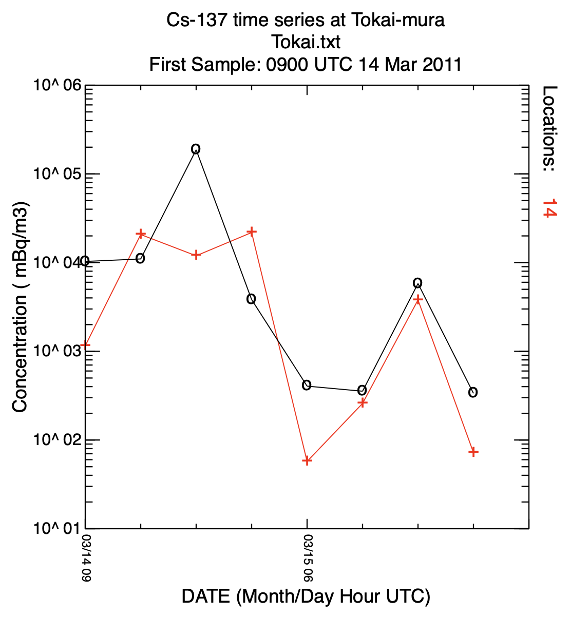
- In the second post-processing step, we create a plot of the total deposition accumulated over the three day simulation period:
concplot concentration plotting program -ifdnpp.bin input HYSPLIT concentration output file -oplot_dept base name of graphic output file +g1 output in SVG such that name={base}.html -h37.0:140.0 location of map center -g0:100 radius of the map -y0.001 convert Bq to kBq -ukBq set units label on map -b0 -t0 process input data from bottom and top level 0 -k2 do not draw contour lines between colors -c4 force contour levels to values after -v -v1000+500+200+100+50+20+10 forced contours from high to low -r3 plot only the total accumulated deposition (last frame) 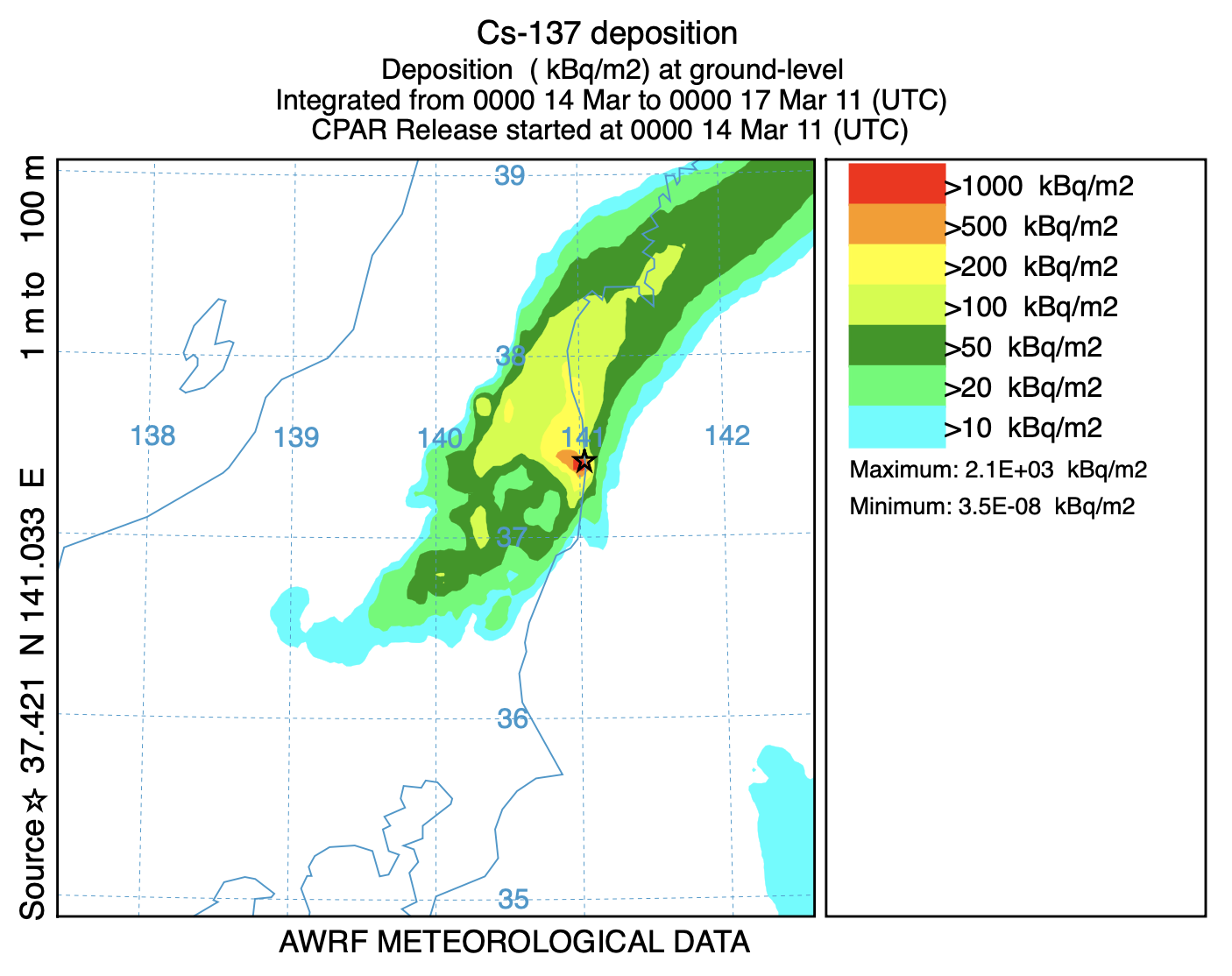
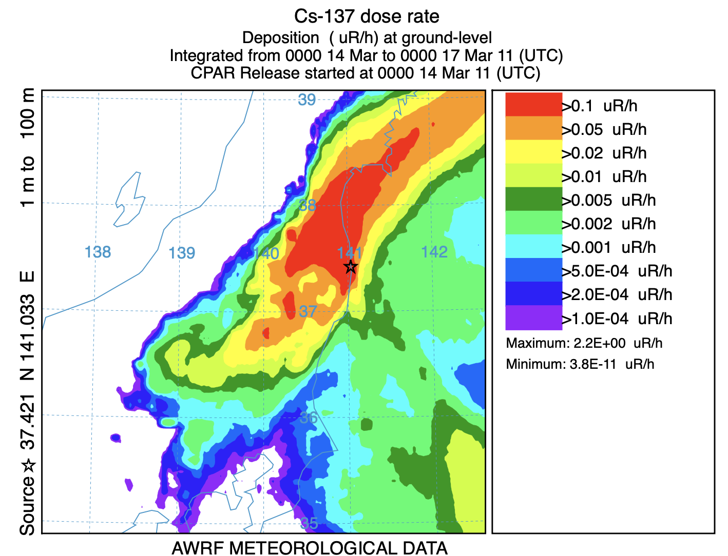
- In the last post-processing step we convert the air concentrations and accumulated deposition at each 3 hour output period to dose using the concentration plotting program. For this conversion we assume that the EPA-DOE dose conversion factors are 3.3x10⁻¹¹ and 1.1E-12 (rem/h per Bq/m3 or per Bq/m2). Only the last time period is shown for deposition and the last time period after emissions have stopped for air concentrations. Note that the total dose would be the sum of of the air and ground components.
concplot concentration plotting program -ifdnpp.bin HYSPLIT binary output file -oplot_dose base name of graphic output file +g1 output in SVG such that name={base}.html -h37.0:140.0 location of map center -g0:100 radius of the map in km -x3.340E-05 convert air concentration to µrem/h -y1.08E-06 convert deposition to µrem/h -k2 do not draw contour lines between colors -c4 force contour levels to values after -v -v0.1+0.05+0.02+0.01+0.005+0.002+ 0.001+0.0005+0.0002+0.0001 forced contours from high to low -r2 sum dose (rate) each time period 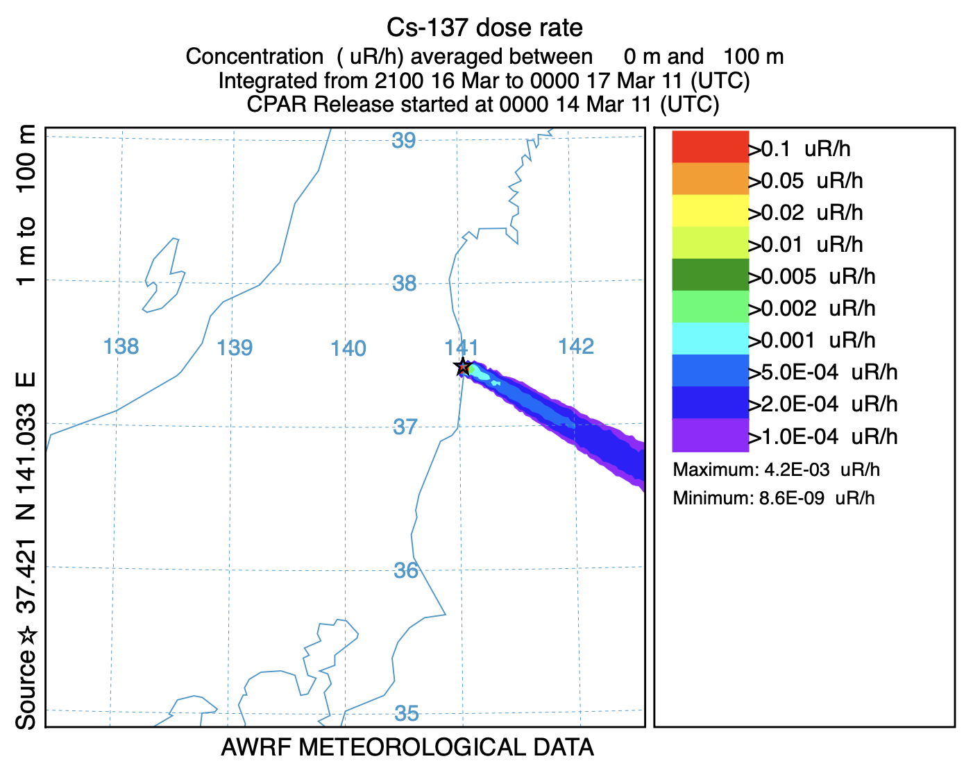
In this simple single-species HYSPLIT radiological configuration, the species characteristics, emission rate, and decay are specified prior to each simulation. Although decay was not considered in this case due to the long half-life of Cesium-137, when decay is calculated during a simulation, once the data have been written to the output file, decay can no longer be applied. This is not an issue for air concentrations, or a exposure calculations where the dose is summed over all the time periods in the file, which permits the use of simple units conversion factors in processing the output. However, if total deposition is required for a short half-life species, its value at the end of the simulation will be an overestimate because the decay was not applied between the time of each output and the end of the simulation.