Multi-species Dose, Constant Emissions
|
||||
 Previous |
|
|
 Next |
|


In previous examples, although one could create an output file with multiple radiological species, the dose computations were limited to a single species using the plotting program conversion factor. In this section we will use the post-processing program CON2REM to compute doses for a more realistic multi-radionuclide emission scenario. The program reads a unit source HYSPLIT concentration file and a file called ACTIVITY.TXT that defines each radionuclide to be included in the dose calculation. In its current configuration, CON2REM supports two computational species; a generic particulate radionuclide RNUC and a non-depositing noble gas NGAS. A dose is computed for each defined radionuclide using either the RNUC or NGAS computations. The dose is defined as the sum of the product of the emissions, dose conversion factor, dispersion, and deposition coefficients over all radionuclides.
- The files required for the simulation (download to your work directory) are the same as the previous example but with one new addition:
wrf11031400.bin WRF meteorological data activity.txt maximum radionuclide emissions for 10 species dose_cemit.sh Script for UNIX/Mac or ... dose_cemit.bat Script MS-Windows
- Two pollutants are required to run this simulation. The simplest approach is to put both on the same computational particle. Add the additional variable line to the standard SETUP.CFG namelist file:
maxdim = 2, define two species on each particle - In addition to setting the output file name to fdnpp_unit.bin, ensure that the emission section of the CONTROL file is set to a unit hourly rate for the duration of the simulation. Two entry sections are required, one for each species:
2 two pollutant definitions follow RNUC generic particulate radionuclide 1.0 emission rate units per hour 72.0 emission duration in hours 00 00 00 00 emission start time (0 defaults to run start) NGAS generic noble gas 1.0 emission rate units per hour 72.0 emission duration in hours 00 00 00 00 emission start time (0 defaults to run start) - The deposition section of the CONTROL file should be configured to correspond to the general characteristics of the RNUC and NGAS pollutants. In the post-processing program only NGAS needs to be defined as a pollutant name. All others are assumed to default to the RNUC pollutant.
2 two pollutant definitions follow 1.0 1.0 1.0 defined as a particle 0.001 0.0 0.0 0.0 0.0 forced dry deposition 0.1 cm/s 0.0 8.0E-05 8.0E-05 below and within cloud wet removal 0.0 no radioactive decay 0.0 no resuspension 0.0 0.0 0.0 defined as a gas 0.0 0.0 0.0 0.0 0.0 no dry deposition 0.0 0.0 0.0 no wet removal 0.0 no radioactive decay 0.0 no resuspension - In the first post-processing step, the model predicted dispersion and deposition factors for the two computational species are converted to dose according to the radionuclides and their emission rates defined in the ACTIVITY.TXT file. Decay is applied to both air concentration and deposition from the start time of the simulation. Nobel gases are identified by the zero value for the ground-shine dose conversion factor and these are all associated with the NGAS dispersion coefficients. All other radionuclides listed are linked with the RNUC dispersion-deposition coefficients. In this example the ACTIVITY.TXT file lists the top-ten radionuclides and their maximum emission rate (Bq/h) during the initial phase Fukushima accident:
con2rem convert concentration to dose -ifdnpp_unit.bin HYSPLIT binary output file -ofdnpp_dose.bin binary output dose file -x66 extend decay time to start at fission stop -d1 compute dose over averaging time (0 = rate) λ = log(0.5) / half-life Decay = [exp(λt) - 1] / λt -aactivity.txt emission rates and dose factors Although not required for this application, because all emission columns are identical, the command line options -f and -p can be used to select the emissions column in the activity.txt file such that Emit1 = f1p1, Emit2 = f1p2, Emit3 = f2p1, and Emit4 - f2p2.
- In the second post-processing step, the ground-shine (deposition level 0) and cloud-shine (air concentration levels 0 to 100) dose values are added together each time period into a combined total dose output:
concsum add ground- and cloud-shine -ifdnpp_dose.bin input binary dose file -ofdnpp_total.bin output binary total dose file -l sum all levels ground+cloud -pDOSE species label in output file - In the third and last post-processing step, the 3-hourly dose values are summed together to obtain a total dose and written to the file as a single output time covering the specified averaging time period:
conavgpd average or sum over time -ifdnpp_total.bin input file of 3-h dose values -ofdnpp_sums.bin binary output file of summed doses -a11031400 YYMMDDHH of summation start -b11031700 YYMMDDHH of summation end -r1 r=1 to sum or r=0 to average - For the first graphics, we produce a time series of the sum of the ground- and cloud-shine dose one would receive at Tokai-mura, about 100 km south of the Fukushima plant. The numbers shown represent the dose each 3-h period and must be accumulated for the total dose:
echo Tokai 36.4356 140.6025 >latlon.txt location to file con2stn extract time series at a location -ifdnpp_total.bin binary dose output file -oTokai.txt text output file at location -slatlon.txt latitude & longitude for each location timeplot time series plot -iTokai.txt input file with data to plot -p2 plot points and connecting lines -y log axis scaling 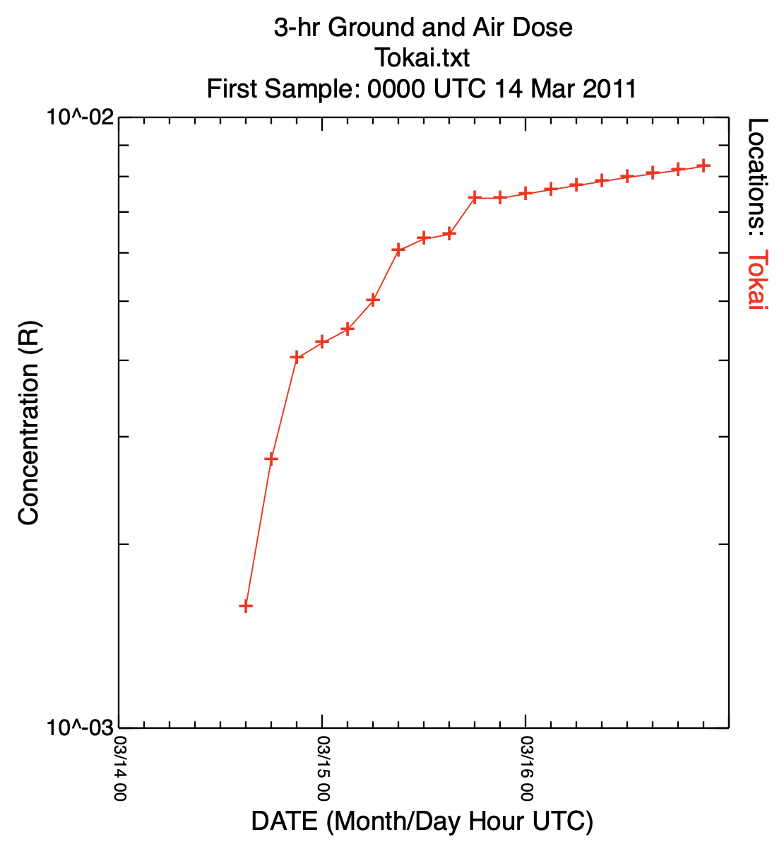
- In the last graphic, we plot the accumulated dose, computed previously, over the entire model simulation period:
concplot concentration plotting program -ifdnpp_sums.bin binary input of dose summation -odose_plot Postscript output file -c4 force contour levels -v1.0+0.3+0.1+0.03+0.01+0.003+0.001 set forced contours 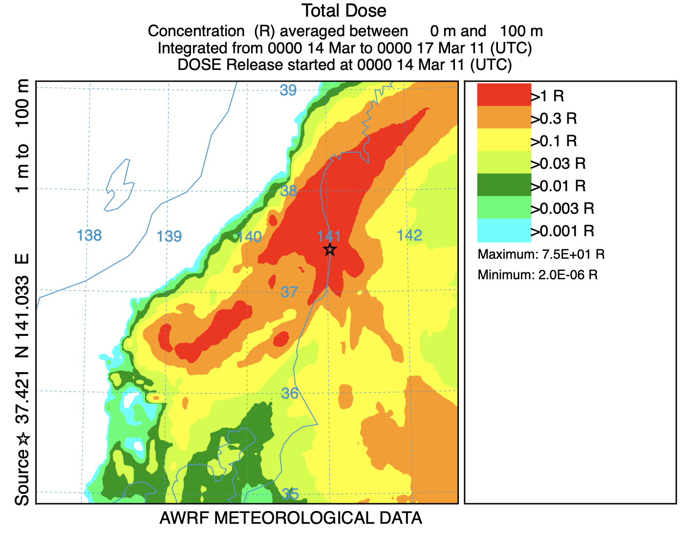
In this HYSPLIT radiological configuration, a continuous unit source dispersion-deposition calculations with two computational species, one representing a small particle and other a noble gas, were run for a multi-day period of interest. Post-processing programs were used to assign each computational species to multiple radionuclides, each with its own emission rate, decay, and dose factors, to compute dose.