Simulation of the Smoky Nuclear Test
|
||||
 Previous |
|
|
 Next |
|


In all the previous examples, we simulated the continuous, although varying in intensity, radionuclide emissions from a nuclear power plant accident. In this example we will configure the model to simulate the transport, dispersion, and deposition of the almost instantaneous emission of radionuclide fission products from the Nevada Smoky nuclear test in August of 1957 and compute the resulting dose. A full description of the modeling effort can be found in an article by Rolph, Ngan, and Draxler (2014) published in the Journal of Environmental Radioactivity. In the following sections we will review the signficant sections of the HYSPLIT configuration required for the simulation.
- Download the following files to your work directory:
meteo_smoky.bin global meteorological reanalysis for 570831 through 570901 activity_smoky.txt activity values and dose factors for 213 radionuclides EMITIMES_smoky.txt emission distribution with height and size for 14 particle sizes smoky_test.sh Script for UNIX/Mac or ... smoky_test.bat Script MS-Windows - The key to the simulation is understanding the EMITIMES emission file. The configuration is based entirely upon the estimated yield of the device, which in this case was equivalent to 44 kT of TNT. The yield determines the vertical height and activity distribution as defined by Heffter (1969) and illustrated in the figure below for a 10 kT explosion example:
For the Smoky test yield of 44 kT, the initial activity distribution of the nuclear cloud is divided into six layers, with the top of the cloud at 12500 m AGL, distributed over 13 particle sizes ranging from 20 to 500 µm according to Glasstone and Dolan (1977). This information is used to create the HYSPLIT emissions file, EMITIMES_smoky.txt for the simulation, with 14 emission rates for each defined layer, one for noble gases and the remaining for 13 different particle sizes.
As in many of the previous radiological simulations, the emission rate should be a unit value, in this case the noble gas value should be one when summed over all release heights, and the sum of the particle emission rates should also be one, but over all particle sizes and heights! Note that the emission rates defined in any EMITIMES file are per hour, and therefore the totals should add up to 60 for gases and 60 for all the particles. Because the emission duration is defined as one minute, the result will be a total emission of one for each. This can be confirmed by examining the total mass in the MESSAGE file at the end of the simulation. The mass starts out with a value of 1.998, just under two, as some particles have already deposited within the first minute. - In configuring the CONTROL file, ensure that the emissions in the are set to zero to avoid using the wrong emission rate in case there are errors in the EMITIMES file. Also set the emission time to 1 minute, which is when the nuclear cloud is considered stabilized. In addition, define the 14 particle diameters, densities, and shapes, making sure the noble gas is defined with all zeroes:
14 14 pollutants (P013-P001, smallest to largest) plus a noble gas (NGAS) 0.0 emission rate units per hour 0.01666667 emission duration in hours (1 minute) - Configure the SETUP.CFG namelist file to define five computational particle size bins centered about each defined particle size (NBPTYP=5) to provide a better distribution of particle sizes for calculating deposition. Also, the mass on a particle is removed once a particle is deposited by having HYSPLIT compute the probability of being deposited when a particle is in the deposition layer (ICHEM=5):
nbptyp=5, number of redistributed particle size bins ichem=5, probability of deposition numpar=15000, particles released per emission cycle (1 minute) maxpar=200000, maximum particle number for array allocation efile='EMITIMES_smoky.txt', unit emissions by particle size and height - Once the HYSPLIT calculations have completed, we display the particle positions every 3 hours of the 24-hour simulation with the final position (+24 h) shown in the illustration below:
parxplot program for a particle cross-section plot -iPARDUMP particle position input file output from HYSPLIT -m1 scale the size of the particle by its activity -n3 plot only every third particle +g1 output format SVG graphic encoded within HTML 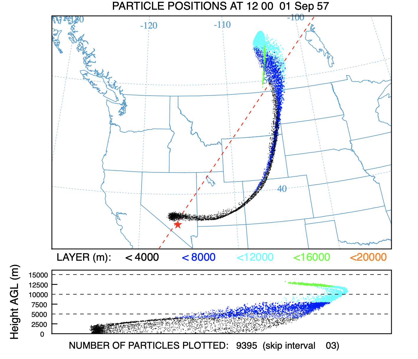
- In the first post-processing step, we convert the HYSPLIT output file of unit source concentrations and deposition for a noble gas and the 13 different particle sizes into dose. The conversion uses the same program con2rem, that was used previously for nuclear power plant accidents, to assign each radionuclide in the activity_smoky.txt file to one of the two computational species, either a gas or particle. Fractionation is not considered and therefore all particulate radionuclides are assigned in the same proportion to all particle sizes. The activity file contains 213 radionuclides
(England and Rider, 1993) present in the nuclear cloud after stabilization, assumed to be about one minute after detonation.
The activity file only needs to be created once to compute the radionuclide yield for various fission reactions. The calculation is based upon the yield per 100 fissions as taken from England and Rider (1993), which has been digitally tabulated. The radionuclide inventories were adjusted using the rate of 1.45x10²³ fissions per kT. The results in the activity file are for a one kT detonation in Becquerels (Bq) for each of the 213 radionuclides, with one column each for 235U and 239Pu, and for high-energy (blast) and thermal (reactor) fissions.
con2rem program converts to dose -ismoky_disp.bin binary input file of HYSPLIT output -osmoky_dose.bin binary output file for dose -aactivity_smoky.txt activity data for each radionuclide -d1 output dose (rather than dose rate) -e1 include inhalation dose -y44.0 yield of weapon (kT) -f1 fuel type is U235 -p1 high energy fission - In the second post-processing step, the ground-shine (from the deposition at level 0) and cloud-shine (from the air concentrations averaged between levels 0 to 100) dose values are added together for all particle sizes (computational species), each time, into a combined total dose output:
concsum program to add ground- and cloud-shine -ismoky_dose.bin input binary dose file by species and level -osmoky_sums.bin output binary total dose file by time all species and levels -l sum all species and levels ground+cloud -pDOSE label in the output file - In the last post-processing step, the hourly dose values are summed together over all the time periods to obtain a total accumulated dose and written to the file as a single output time covering the specified integration time:
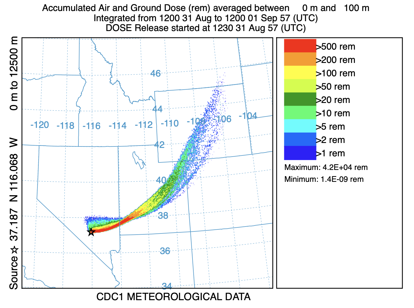
conavgpd program to average or sum over time -ifdnpp_sums.bin input file of hourly dose values -ofdnpp_accd.bin binary output file of accumulated doses -r1 r=1 to sum (or r=0 to average) - Finally display the accumulated dose map after 24 hours, at the end of the simulation:
concplot concentration plotting program -iaccd.bin HYSPLIT binary output file -osmoky_accd.html Postscript output file -c4 force contour levels +g1 output SVG graphic within an HTML file -k2 do not draw contour lines between colors -v500+200+100+50+20+10+5+2+1 forced contour values - For these types of events, besides the accumulated dose, there may be some interest in determining the dose rate after 24 hours or even longer periods to determine if it might be safe to return to an affected area. In this case we would only care about the ground shine dose because the air dose contribution would have been dispersed and transported downwind. The existing HYSPLIT output file can be converted to dose rate in three steps:
- con2rem -d0 -y44.0 -f1 -p1 -x0
- concsum -pDOSE
- concplot -n24:24 -b0 -t0
Left as an exercise, modify the script to show the dose rate after a week (-x144), and you should get the following result, now showing a maximum rate of 0.34 rem/h.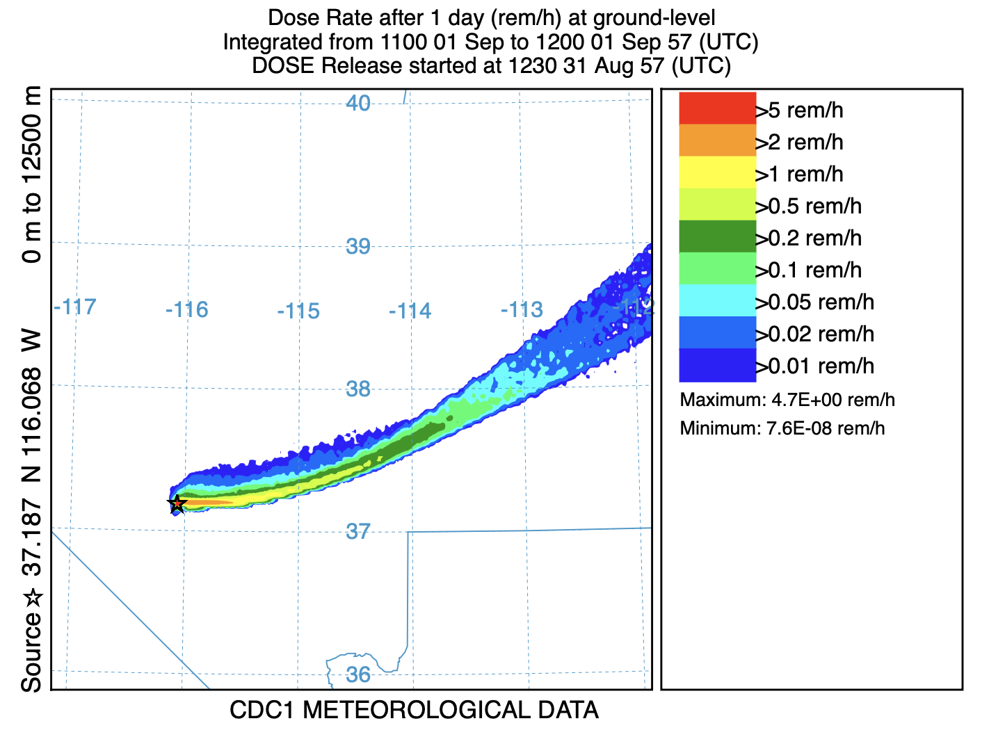
It is not necessary to rerun the entire calculation, but the computational aspects of the script can be disabled and the original HYSPLIT calculational results can be reused. Although we added 6 days to the decay calculation, the time label on the plot, 1 September, is identical to the previous graphic. The HYSPLIT output times are not affected by adjustments to the decay times. HYSPLIT could be run very quickly for a week, when there are no particles left, to generate the proper output times in the computational file for display.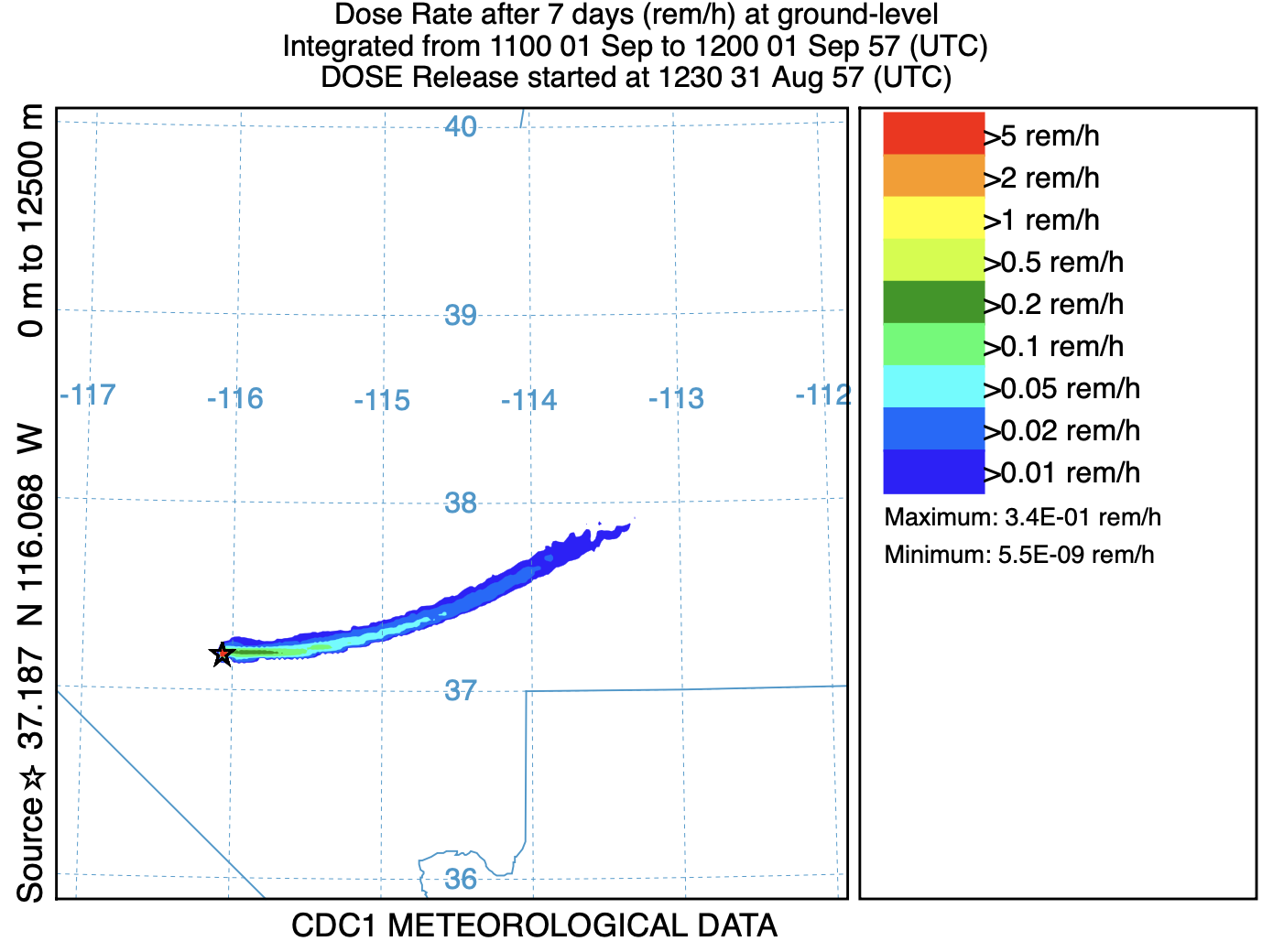
Although an earlier version of this example showed a more complex sequence of calculations with many more intermediate files, in this example, the simulation of the Smoky test was reduced to just the most essential elements, showing how the same HYSPLIT tools that were previously used to simulate the continuous emissions from a nuclear power plant accident, can be applied to the instantaneous emissions that result from the detonation of a nuclear device.