Comparing the True Trajectory with HYSPLIT |
||||
Home |
||||
The WINDMAKE program uses the equations derived by Lester Machta in an unpublished 1958 manuscript titled "A Mathematical Verification of Trajectory Methods" by defining a sinusoidal variation of the south-north wind component superimposed on a constant west-east zonal current, which is then used to create a gridded meteorological data file. This file can then be read by HYSPLIT to compute trajectories. In addition, an analytic form of the trajectory equation using the parameters for the sinusoidal wind field is solved to provide the "True Trajectory" and which is written to an output file compatible with the HYSPLIT trajectory plotting program. The WINDMAKE program, in conjunction with the results from HYSPLIT, can be used to explore the effects sparse grids in space or time on the accuracy of trajectories integrated using gridded data versus the analytic true solution to the trajectory, which uses a continuous representation of the wind field.
- Following Machta (1958), the windmake program defines the wind field as:
- U = constant
- V = A sin 2π (x - ct) / L
and where U is the zonal west to east wind speed, V is the south to north wind speed, A is the maximum value of V, L is the wavelength, c is the west to east wave speed, and t is time. The solution for the true trajectory for this wind field is then:
- x = Ut + x0
- y = AL [cos 2πx0/L - cos 2π {x0 + (U-c) t} / L ] / [2π (U-c)] + y0
where x0,y0 is the initial trajectory position. The windmake program is not part of the HYSPLIT distribution, but the source code and executables for a few operating systems are available for download. - To understand the required program data entries and the resulting output, a demonstration is the best approach. To simplify the link with HYSPLIT, place the executable in the hysplit/exec directory. Then from the HYSPLIT working directory type ./windmake. The following entries will show the results for the default example. Note that all entries have an initial [default] value. If the default has a decimal point, enter your value with a decimal point. If not, then none is needed. Also, if you want to accept the default, just enter a forward slash, /, followed by the return key.
- Zonal wind U component in meters per second [1.0]
- Maximum amplitude of the V component in meters per second [2.0]
- Wavelength of the sinusoidal variation in kilometers [100.]
- West to east speed of the wave in kilometers per hour [0.0]
- Duration of the trajectory calculation in hours [28]
- Trajectory endpoint output interval in minutes [60]
- Trajectory starting position within the sine wave in degrees [90.0]
- Meteorological grid extent in the number of wavelengths [2.0]
- Distance between the grid points in kilometers [5.0]
- Meteorological data grid output interval in minutes [60]
- The windmake program creates several output files:
- windtraj.txt - contains the hourly endpoint positions of the analytic trajectory solution in the HYSPLIT trajectory plot format.
- CONTROL - the control file required for the HYSPLIT simulation that would correspond with the analytic trajectory.
- windgrid.bin - the HYSPLIT compatible meteorological data file with the sinusoidal wind field that was used to compute the analytic trajectory.
The CONTROL file is the key to making the connection between the two approaches. It translates the starting trajectory position along the sine wave into the latitude-longitude required for HYSPLIT calculations. This conversion is simplified by assuming that the analytic solution coordinates of x=y=0 corresponds to the HYSPLIT coordinates of latitude=longitude=0 and at the equator distance in longitude is equivalent to distance in latitude. The CONTROL file also defines a default trajectory output file name of hysptraj.txt which would then be compared with the analytic true solution file windtraj.txt.
- After windmake completes open the HYSPLIT GUI, go to the Trajectory Setup menu, retrieve the CONTROL file created by windmake, save, and then run HYSPLIT. After it completes open the trajectory display menu, and to the end of the endpoints file hysptraj.txt add +windtraj.txt, the analytic results. Set the time label to hourly and then display the resulting trajectories:
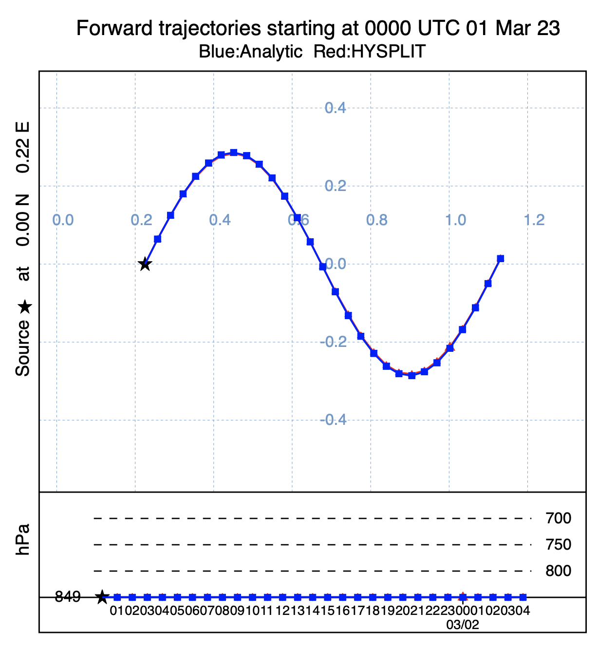
The default example shows two sine wave like trajectories superimposed on each other. The red is the HYSPLIT trajectory, the first file is always red, while the blue one represents the true trajectory, the analytic solution for the wind field. They are identical. There is no error in the HYSPLIT numeric solution. - With windmake it is easy to test various modeling assumptions. For instance, the effects of decreasing spatial resolution on the accuracy of the numerical integration of the trajectory position. Rerun windmake again with all the defaults, except increase the meteorological data file grid size from 5 to 80 km, run HYSPLIT, and display the two trajectories:
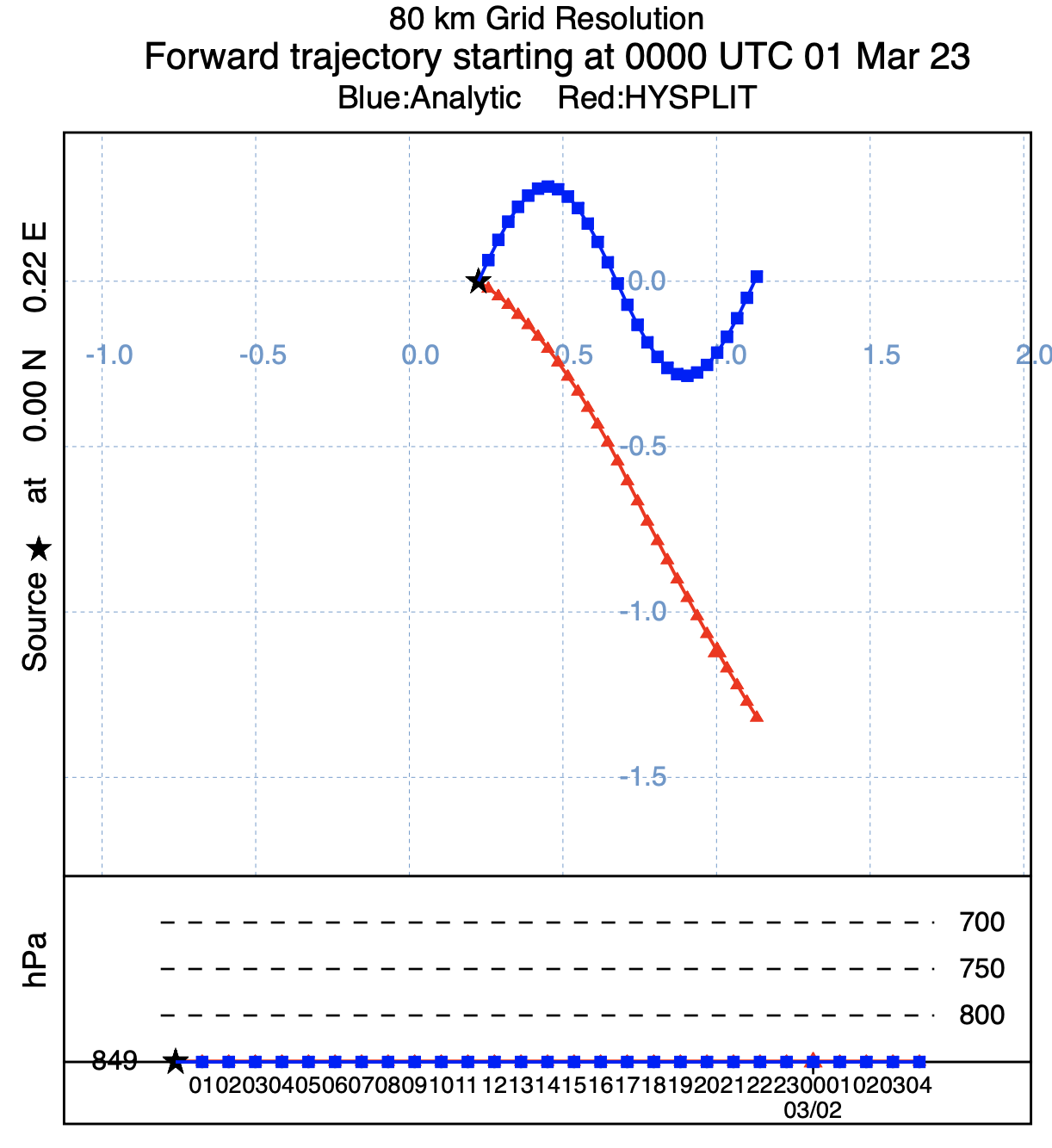
which clearly shows the error systematically increases with time. At 80 km resolution, close to the wavelength of the wind-field, the trajectory integration using the gridded data suffers from insufficient spatial resolution to reconstruct the details of the flow.
At this point one might ask if the windmake program has any practical value. It might be possible to define the sine wave characteristics of the wind field for a small region, but it is quite likely that those values would change over time. The main value of this program is that it provides an opportunity to deconstruct the trajectory calculation into its basic components and to improve one's understanding of how the limits in the meteorological data, in terms of its spatial and temporal resolution, can affect the accuracy of the numerical trajectory integration.