Daily Forecast with a Transfer Coefficient Matrix

In a previous radiological example we updated a Transfer Coefficient Matrix (TCM) by merging individual short-duration simulations for each release period and sampling period to create a single air concentration-deposition output file. It was noted without explanation that during a real-time event, HYSPLIT can be configured to provide a continuous update to the TCM with each new forecast cycle by using the current-time particle positions to create a dispersion forecast. In this example, we will review how that script can be modified to provide daily updates to the dispersion forecast for such a continuous source event.

• The forecast meteorological files required for the simulation (hysplit.t00z.namsf.NEtile) are no longer available on the server. Forecasts are deleted after a few days. However, the script should work with any three sequential 00Z forecasts. The forecast files should be renamed {base}{DD}.t00z. See the script for details.
  

  NAM07.t00z		Meteorology Forecast for the 7th and 8th
  NAM08.t00z		Meteorology Forecast for the 8th and 9th
  NAM09.t00z		Meteorology Forecast for the 9th and 10th
  tcm_daily.sh		Example script

• The previous example was configured for a radiological event. For this example that script was simplified to its most basic elements, the dispersion of a non-depositing inert gas. For this hypothetical event a continuous emission is assumed which is divided into six hour computational segments. The event starts at 00 UTC 7 January. The script is run three times, once each day when the 00 UTC forecast becomes available. Each daily forecast, expressed as an air concentration output, extends out to 48 hours. On the second day, the four emission periods that occurred on day one, 00-06, 06-12, 12-18, and 18-00, are continued into day 2 using the meteorological data from 00 UTC 8 January, replacing all the output files from 8 January. During the day 2 simulation, the day 1 output files are not affected. The process is similar for the day 3 simulation, 9 January, where the day 1 and 2 results are unaffected, but the new forecast extends out through 10 January. This sequence can continue for the entire duration of the emission event.


• At the start of the script enter the two-digit year, month, and day of the 00 UTC forecast that will be used in the calculations.
  
  Starting time of forecast and emission
  Enter year YY?
  Enter month MM?
  Enter day DD?


• The initial simulation question is the most important. (Y)es means it is the start of the event and all the temporary and intermediate files from any previous calculations will be deleted. A (N)o response means that this is a continuation of a previous event. A continuation means that the list of simulation start times from all previous days will be copied to the start_list.txt file. These are the simulations that will be initialized from their particle files and continued into the new forecast period. Also all of the new emission start times will be added to the list as the script is executed.
  
  Initial Simulation (y/n)?



• The script then proceeds in a manner similar to all the other HYSPLIT scripts, configuring the required files ASCDATA.CFG, SETUP.CFG, and all necessary internal script variables:
  

  olat=48.0		Emission point latitude
  olon=-88.0		Emission point longitude
  lvl1=10.0		Emission height above ground level
  run=6		Simulation duration in hours
  data=NAM		Base name of the meteorological data

  
  The emission location can be set to any location covered by the meteorological data. The simulation duration can be changed, but it should correspond with the number of simulations per day hardwired into the script to insure a continuous emission. Note that in a subsequent script section, the output averaging interval is also set to 6 hours. However, that value is independent of the simulation duration.



• The SETUP.CFG namelist file should contain the variables needed to insure a sufficient particle release rate given the duration of the emissions and the resolution of the concentration grid. In addition, the particle positions should be output to a file at the end of each simulation, which we have defined earlier to be 6 hours:
  

  ndump = ${run}

  Particle positions are output at this interval

  
  Also in this case we are using a regional meteorological extract, so that particles will be terminated when they reach the grid boundary. For simulations using global meteorological data, but where the interest is still regional, it may be desirable to also define a maximum particle age using khmax.



• The next section of the script defines a loop where each iteration represents a new emission start time within the two day forecast period. If the run duration were to be changed from 6 hours then a corresponding change is required in the start times of the HH loop. Within that loop there are two parts. In the first part HYSPLIT may be run multiple times; there is one simulation for each previous emission as tabulated in the file start_list.txt. The second part consists of one more simulation, for the new emission that corresponds to the DD and HH iteration of the loop. Once a new emission has occurred, its start time is added to the start_list.txt file.
  

  for fd in 0 1; do		Two day forecast loop
  let dd=$sd+$fd		Relative to absolute day
  DD=`printf %2.2d $dd`		Insure two digit days
  for HH in 00 06 12 18; do		Start times every 6 hours
  cat start_list.txt | while read PRUN; do		Set DDHH for each previous run
  ...create CONTROL; run HYSPLIT		Continuation simulations
  done
  create CONTROL; run HYSPLIT		New emission simulation
  echo ${DD}${HH} >>start_list.txt		Update list with the new emission time



• Expanding further on those two parts discussed above, there will be two CONTROL files, one for each part. In the first, the particle restart simulation, no new particles are released, and the release rate is zero for a duration of zero hours. Any particles in that calculation would have been carried forward from the previous calculation for the release times defined in the start_list.txt file. In the second part, the CONTROL file defines a new particle release with a unit source rate for six hours. In both parts, the name of the concentration output file (CG_*) should reflect the release time and sample start time, but in the first part, the release DDHH is taken from the list of previous emissions (PRUN), while in the second part, the release DDHH is equal to the sample start DDHH.
  
  
  1. Re-start Simulation (no particles released)

     GASP		Defined as a GASeous Pollutant
     0.0		Emission rate in units per hour
     0.0		Emission duration in hours each cycle
     CG_${smo}${DD}${HH}_${DD}${HH}		Release start and sample start times

  
  
  2. New-start Simulation (particles released)

     GASP		Defined as a GASeous Pollutant
     1.0		Unit emission rate per hour
     ${run}.0		Emission duration 6.0 hours each cycle
     CG_${smo}${PRUN}_${DD}${HH}		release start = sample start time

  
  
• At the end of every simulation a particle output file needs to be created. This file will then be used to initialize the next stimulation in the time sequence for that release. In the script described here, computations are performed at 6 hour intervals. In the first 0-6 hours there would only be one simulation. Between hours 6-12 there would be two, a continuation of the 0-6 simulation, and one with new emissions. During hours 12-18 there would be three simulations, two continuations with no new emissions, and again one with new emissions. The continuation simulations are initialized with the particle output file from its predecessor. At the end of each HYSPLIT simulation, for part 1 or part 2, the PARDUMP output file is renamed to correspond to the emission time for that simulation:

  mv PARDUMP PARDUMP_${PRUN}		Part-1 Re-start simulation
  mv PARDUMP PARDUMP_${DD}${HH}		Part-2 New-start Simulation



• Prior to every re-start simulation, the particle output file for that release time needs to be renamed to the default name PARINIT which is used to initialize HYSPLIT. In the situation where the script is run for the first time for a release, particle initialization is not needed. Previous simulations (Part 1) are identified by the DDHH written in the start_list.txt file which is then used to identify the correct file to open:
  
  mv PARDUMP_${PRUN} PARINIT
  
  This works fine for the initial execution of the script. However, on the second execution the script, when new forecast data become available, the contents of all the PARDUMP_${PRUN} files will reflect the particle positions +48 hours after the start of the event, while in our case, we are restarting the script at +24 hours. Therefore, we retain the Particle Position data for each simulation, prior to starting HYSPLIT, by copying each file to a standard name (PP_) corresponding to the release and sample time.
  
  cp PARINIT PP_${smo}${PRUN}_${DD}${HH}
  

  The PP files are used at the beginning of the script to insure that each restart simulation listed in the start_list.txt file contains the particle positions that correspond to the respective release and simulation start time.
  
  cat start_list.txt | while read PRUN; do
  ... mv PP_${smo}${PRUN}_${sda}${shr} PARDUMP_${PRUN}
  



• The 6-hour simulations for each release and sampling period for the above example would have created 136 CG_{MMDDHH}_{DDHH} files which represent 16 release periods over four simulation days (7,8,9-10). In the next step these files are combined into one file per release period that contains all the sampling periods. This is accomplished using another loop to go through each release time and find all the sampling files for that release time and then use the standard HYSPLIT library program CONAPPEND to merge the files in the list to a single file named TG_{MMDDHH}. There will be a total of 16 TG files, one for each release time.
  
  cat start_list.txt | while read PRUN; do
  ... emit=`cat emit_${smo}${PRUN}`
  ... ls CG_${smo}${PRUN}_???? >conc_list.txt
  ... ${MDL}/exec/conappend -iconc_list.txt -oTG_${smo}${PRUN} -c${emit}
  

  A simplification introduced into this script demonstrates how one could apply time varying emissions. In this case conappend is run with a concentration multiplier value ${emit} which is read from a file named emit_${MMDDHH}, where the date field corresponds to the emission time. This file is created after each new unit-source release HYSPLIT simulation. In this example, each file contains a release amount of 10¹² µg, which would result in air concentration output of µg/m3. In a real case, the creation of this file would be disabled and values for the real-event would be provided instead.



• The final step is to merge the individual release files into a single file using the program CONMERGE. The procedure is similar to the CONAPPEND application. The final result is a single file hysplit.bin that contains all releases and sampling periods using the defined emission profile.
  
  ls TG_?????? >merg_list.txt
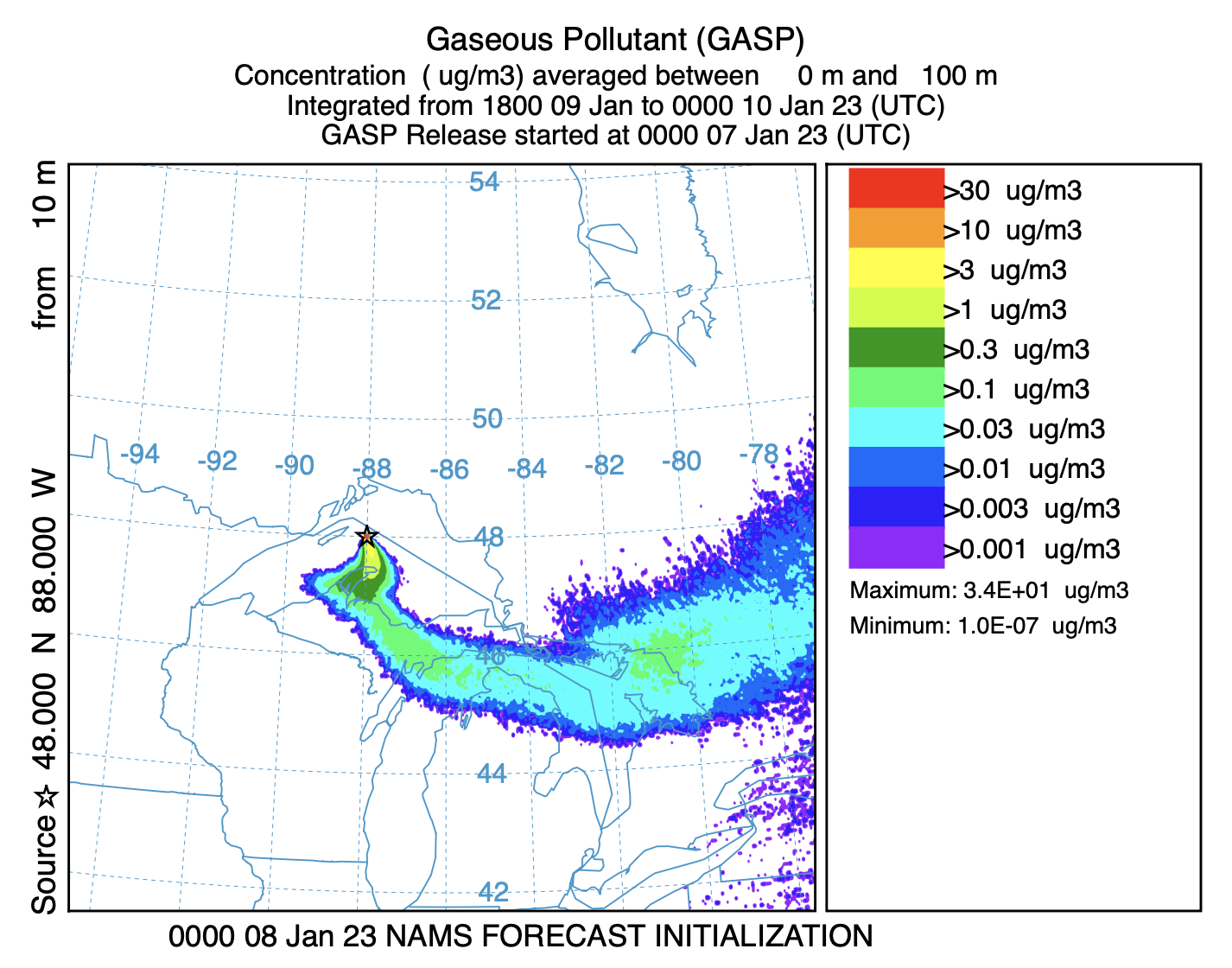
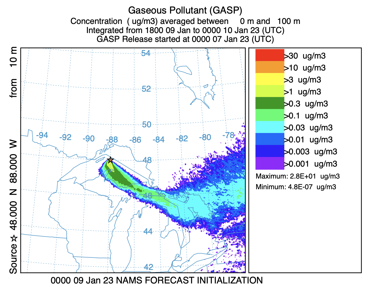
  ${MDL}/exec/conmerge -imerg_list.txt -ohysplit.bin



• For this example, the script was run three times, initially for 7 January 2023, then again for the 8th, and 9th. The output graphic from each simulation contains 8 frames, at 6 hour intervals out to a +48 h forecast. The two graphics below illustrate the nature of the output product. The left frame is from the simulation starting on the 8th, the last frame of the graphic, a +42 to +48 hour forecast, representing the time period 1800 on the 9th through 0000 on the 10th. The frame on the right is from the simulation on the 9th, showing the same output time period, 1800 on the 9th through 0000 on the 10th, but this time it is frame number four of the output graphic, representing the +18 to +24 h forecast. There are some slight differences between the shorter and longer forecast times.

This unit described how a TCM can be computed incrementally as the release progresses, updating the particle position from previous releases with each meteorological data update. The update process is trivial to parallelize because each release simulation is independent of the others and can be computed simultaneously on multiple processors. Note that the example script is only a template that still requires some customization for a specific event.